Introduction

If you have used TensorFlow before, you know how easy it is to create a simple neural network model using the Keras API. Just create an instance of the Sequential model class, add the number of desired layers and accompanying layer nodes, define the activation functions to be used by each layer, and compile your model by providing an optimizer and loss function.  Right? While this process is simple enough to grasp conceptually, it can quickly become an ambiguous task for those just getting started in deep learning.

Why does the output layer take a different shape between a regression and classification problem? Is there a reason why one online tutorial solved a binary classification problem using a network with only one node in the output layer, while another tutorial solved the same problem using two nodes? And, what about the activation function on the final layer of a network when performing classification – why is there a softmax and sigmoid? Do I really need to specify a different loss function for different types of classification problems?

Regression

When developing a neural network to solve a regression problem, the output layer should have exactly one node. 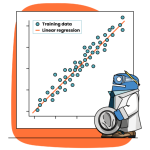Here we are not trying to map inputs to a variety of class labels, but rather trying to predict a single continuous target value for each sample. Therefore, our network should have one output node to return one – and exactly one – output prediction for each sample in our dataset.

The activation function for a regression problem will be linear. This can be defined by using activation = ‘linear’ or leaving it unspecified to employ the default parameter value activation = None.

>>> import tensorflow as tf
>>> model = tf.keras.models.Sequential()

# Define internal model architecture
>>> model.add(...)
>>> model.add(...)

# Define output layer; all of the below are equivalent
>>> model.add(tf.keras.layers.Dense(units=1, activation='linear'))
>>> model.add(tf.keras.layers.Dense(units=1, activation=None))
>>> model.add(tf.keras.layers.Dense(units=1))

>>> a = tf.keras.layers.Dense(units=1, activation='linear')
>>> b = tf.keras.layers.Dense(units=1, activation=None)
>>> c = tf.keras.layers.Dense(units=1)

>>> a.activation([1,2,3])
[1, 2, 3]
>>> b.activation([1,2,3])
[1, 2, 3]
>>> c.activation([1,2,3])
[1, 2, 3]

Evaluation Metrics for Regression

In most cases, the loss function for a regression problem will be the Mean Squared Error (MSE). 

Other metrics can be reported and evaluated during the model training and testing phases by providing a list of metrics to the model.compile() command. Popular reporting metrics include:

• Root Mean Squared Error (RMSE) – a good option if you’d like the error to be in the same units as the target variable
• Mean Absolute Error (MAE) – useful for when you need an error that scales linearly
• Median Absolute Error (MdAE) – de-emphasizes outliers

Classification

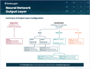
When it comes to classification things get a little more complicated. There are three main types of classification problems to consider when training neural networks–each with its own types of configurations.

Binary Classification

Binary classification describes a scenario where the target is a class of binary outputs – an array of 1s and 0s. In this case, we are trying to create a model that will accurately predict between two – and only two – class labels.

When it comes to binary classification, the way our data is stored determines the choices for the output layer configuration. Consider the following datasets that describe the same problem: whether or not a machine is in a failure state (y) considering a set of input features (X). Notice that one format of y has a single vector of integers (Failure State) while the other format of y has a matrix of One-Hot-Encoded (OHE) integers to represent both states of the machine (State: Success and State: Failure).

X (Feature Matrix)				y (target)		y (OHE target)
Uptime	Temperature	Load		Failure State		State: Success	State: Failure
2987	38	0.87		1		0	1
2719	22	0.03		0		1	0
960	27	0.24		0		1	0
1224	34	0.76		1		0	1
877	37	0.94		1		0	1
1139	23	0.42		0		1	0
1373	32	0.54		1		0	1

If your data has a target that resides in a single vector, the number of output nodes in your neural network will be 1 and the activation function used on the final layer should be sigmoid. On the other hand, if your target is a matrix of One-Hot-Encoded vectors, your output layer should have 2 nodes and the activation function on the final layer should be softmax.  

The reason for the differing activation functions relates to the number of nodes in the final layer of your model.  When dealing with classification problems, it is best to have the output of your network be a representation of a probability distribution. What does this mean? Consider the raw output of a classification network using the table above to be [30, -2, -10, 0.1, 1, -30, 20] — one prediction for each sample (or row in the table). These numbers are essentially meaningless information until transformed into a state that can be used to make a classification prediction. The activation function on the output layer alters this raw data in a way that allows us to interpret the resulting numbers as probabilities.

>>> print(logits.numpy())
[ 30.   -2.   -10.   0.1   1.   -30.   20.]

>>> sigmoid_out = tf.keras.activations.sigmoid(logits)
>>> print(sigmoid_out.numpy())
[1.   0.11920291   0.0000454   0.5249792   0.7310586   0.   1.]

The raw output from the final layer of the neural network has now been transformed into a probability for each class. By using the sigmoid function, we can now interpret the output as a probability distribution and mark all predictions greater or equal to 0.5 as being classified as 1 and all predictions less than 0.5 as being classified as 0.

>>> print(tf.cast(sigmoid_out >= 0.5, tf.int32).numpy())
[1 0 0 1 1 0 1]

Notice that the output of the sigmoid function assumes a probability distribution relating to only one class – each output probability must be compared to a threshold value to determine whether or not the prediction belongs to class 1. In this case, we use the condition >= 0.5 means class 1 and < 0.5 means not class 1 (i.e., class 0).

In the case where the data is stored in OHE format, and the final layer has 2 nodes, a sigmoid function cannot be used and instead the softmax function is employed. The sigmoid function is actually equivalent to a 2-element softmax, where the non-output element is assumed to be zero.

>>> print(logits.numpy())
[[  0.   30. ]
 [  0.   -2. ]
 [  0.  -10. ]
 [  0.    0.1]
 [  0.    1. ]
 [  0.  -30. ]
 [  0.   20. ]] 
>>> softmax_out = tf.keras.activations.softmax(logits)
>>> print(softmax_out.numpy())
[[0.         1.        ]
 [0.880797   0.11920291]
 [0.9999546  0.0000454 ]
 [0.4750208  0.5249792 ]
 [0.26894143 0.7310586 ]
 [1.         0.        ]
 [0.         1.        ]]

>>> print(softmax_out.numpy().argmax(axis=1))
[1 0 0 1 1 0 1]

Notice that the output of the softmax function generates a probability distribution relating to each class – each output has a probability relating to class 0 and class 1. In this case, we use the argmax() method to find which of the two classes has the highest probability and choose that as the predicted class. The sigmoid function will assume output probabilities should relate to only one class (hence the use of only one node in the output layer) while the softmax function will assume probabilities need to relate to each class in the target variable. For the binary classification case, that means two classes, and thus two nodes are used in the output layer.

# Binary classification output layer
# Target stored in single data vector
>>> model.add(tf.keras.layers.Dense(1, activation='sigmoid'))

# Binary classification output layer
# Target stored as OHE vectors
>>> model.add(tf.keras.layers.Dense(2, activation='softmax'))

The loss function used for binary classification problems is determined by the data format as well. When dealing with a single target vector of 0s and 1s, you should use BinaryCrossentropy as the loss function. When your target variable is stored as One-Hot-Encoded values, you should use the CategoricalCrossentropy loss function.

Switching from a target that is represented as a single vector of integers to a OHE encoded matrix is easy as using tf.utils.to_categorical().

>>> print(single_vector_target.numpy())

[1 0 0 1 1 0 1]

>>> print(tf.keras.utils.to_categorical(single_vector_target))
[[0. 1.]
 [1. 0.]
 [1. 0.]
 [0. 1.]
 [0. 1.]
 [1. 0.]
 [0. 1.]]

A final layer with 2 nodes or 1 node is a matter of preference. However, each architecture has its advantages and disadvantages.  Choosing to use 1 node for the output layer results in less work for the model (less weights to learn) but leads to more manual work as prediction probabilities must be converted to class predictions (where >= 0.5 yields a class 1 prediction and < 0.5 yields a class 0 prediction). Choosing to use 2 nodes will require more weights to be learned during model training, but lends to a more interpretable result as the output can be readily used as probability distribution between two classes.

Multi-Class Classification

Multi-class problems aim to predict a single class label from a set of mutually exclusive class labels. When we are in a multi-class scenario,

the number of nodes in the output layer will always match the number of classes in our target variable. For example, if our target variable contained the noble gasses from the periodic table, the output layer of our model would have exactly 6 nodes – one for each gas: Helium (He), Neon (Ne), Argon (Ar), Krypton (Kr), Xenon (Xe), or Radon (Rn).

As the activation function in the final layer for a multi-class problem will always be a softmax, the only difference in configuration lies in which loss function to choose. TensorFlow has two different loss functions for multi-class classification and the choice is determined by the format of the data. SparseCategoricalCrossentropy computes the cross-entropy between the target and predictions when there are two or more labels within the target class. This loss function expects the labels to be provided as integers in a single vector. If the target variable has labels in the one-hot representation, CategoricalCrossentropy must be used. There is an important distinction between these two losses and needs to be considered when compiling your model for training. Remember to choose the correct corresponding cross-entropy based on your target variable’s data layout.

Multi-Label Classification

The goal of multi-label classification problems is similar to multi-class problems except that target labels are no longer mutually exclusive. In a multi-label scenario, the goal is to capture all the labels for a given entity as accurately as possible. Using the chemical elements example again, if we wanted to predict the traces of all noble gasses in an environment, we would no longer want to predict a single gas out of the available options. Instead, we would want to predict a probability of presence for each gas out of the available options.

# Multi-class scenario
# Predictions for five samples; target is ONE of six noble gasses
>>> print(softmax_out.numpy())
[[0.02479219 0.02803683 0.01173518 0.54410144 0.3816906  0.00964376]
 [0.09599111 0.36037244 0.10256758 0.06220797 0.29186875 0.08699215]
 [0.22594247 0.29207357 0.32014403 0.04116754 0.10774433 0.01292806]
 [0.12367229 0.68514548 0.02211832 0.01085471 0.1388765  0.01933271]
 [0.03213059 0.02881347 0.04113723 0.59102145 0.07266653 0.23423073]]

# All rows sum to 1
# Each row is a probability distribution between 6 classes
>>> print(softmax_out.numpy().sum(axis=1))
[1. 1. 1. 1. 1.]

# A single noble gas is selected based on the highest probability
>>> print(targets)
['He' 'Ne' 'Ar' 'Kr' 'Xe' 'Rn']
>>> print(softmax_out.numpy().argmax(axis=1))
[3 1 2 1 3]
>>> print(targets[softmax_out.numpy().argmax(axis=1)])
['Kr' 'Ne' 'Ar' 'Ne' 'Kr']

# Multi-label scenario
# Predictions for five samples; target is a COMBINATION of noble gasses
>>> print(sigmoid_out.numpy())
[[0.25036845 0.27415201 0.13650989 0.87995023 0.83718542 0.11497865]
  [0.36691149 0.68511794 0.38243554 0.27303821 0.6379688  0.3443593 ]
  [0.56733358 0.62894784 0.65009822 0.19284173 0.38472538 0.0697913 ]   
  [0.6757269  0.92028304 0.27149984 0.15461767 0.70059917 0.24570835]
  [0.2895576  0.26766553 0.34289295 0.88231215 0.47964595 0.74818668]]

# All rows do not sum to 1
# Each value in a row is a binary probability for presence of a gas
>>> print(sigmoid_out.numpy().sum(axis=1))
[2.49314465 2.68983128 2.49373805 2.96843497 3.01026086]

# The presence of each noble gas is selected based on binary threshold
>>> print(tf.cast(sigmoid_out.numpy() >= 0.5, tf.int32).numpy())
[[0 0 0 1 1 0]
 [0 1 0 0 1 0]
 [1 1 1 0 0 0]
 [1 1 0 0 1 0]
 [0 0 0 1 0 1]]
>>> preds = tf.cast(sigmoid_out.numpy() >= 0.5, tf.int32).numpy()
>>> [tuple(targets.compress(pred_row)) for pred_row in preds]
[('Kr', 'Xe'), ('Ne', 'Xe'), ('He', 'Ne', 'Ar'), ('He', 'Ne', 'Xe'), ('Kr', 'Rn')]

This is like fitting multiple binary classification problems at once–one for each target class. Notice that the multi-class scenario has an entry for each corresponding noble gas and that each row will sum to 1. A single noble gas is selected based on the highest probability within a given row.

The multi-label scenario has a value for each noble gas, however, each row does not sum to 1. Instead, a separate binary classification is run for each of these values per row. This shows how a multi-label problem can identify more than one label for a given sample: by classifying instances that have a value greater than or equal to 0.5 as 1 and those values less than 0.5 as 0. As the multi-label problem fits binary classifications for each class in the target variable, it should follow the binary classification case closely. The number of nodes in the final layer should be equivalent to the number of classes in our multi-label problem and the activation function of our output node should be sigmoid.

The target variable for multi-label classification problems cannot be represented in a single vector of integers nor can it be represented in the One-Hot-Encoded format. These problems need to have target variables that have been binarized – each sample’s target is represented by a row in a 2d array of shape (n_samples, n_classes) with binary values where the non-zero elements correspond to the subset of labels for that sample. As shown above, [1 1 0 0 1 0] represents the presence of  (‘He’, ‘Ne’, ‘Xe’) given targets of [‘He’ ‘Ne’ ‘Ar’ ‘Kr’ ‘Xe’ ‘Rn’]. Since the target variable must be represented in this way, and the fact that a single binary classification will be performed per target class, it is like saying our data is in a single data vector containing 1s and 0s per target class. This leads to the conclusion that BinaryCrossentropy should be used as the loss function for multi-label classification problems.

Evaluation Metrics for Classification

When considering classification, cross-entropy is the most popular choice for a loss function.  Cross-entropy is a measure of the difference between two probability distributions. We want to minimize the difference between the model’s predicted probability distributions and those of the training dataset. However, the interpretation of cross-entropy is usually not readily apparent to most practitioners. Instead, a measure like accuracy is much more interpretable.

Other metrics like accuracy, area under the receiver operating characteristic curve (AUC), precision, and/or recall can also be used to interpret the performance of a model.  Accuracy calculates how often predictions equal labels (number correct over total). Unfortunately, there are several accuracy metrics within TensorFlow that can yield different results when fitting a model. It is possible to use metrics=[‘accuracy’] when using model.compile() but this could yield unexpected results as Keras will guess which accuracy to use, depending on the loss function you specify. It’s best to be explicit here.

• tf.keras.metrics.Accuracy: Calculates how often predictions equal labels
• tf.keras.metrics.BinaryAccuracy: Calculates how often predictions match binary labels.
• tf.keras.metrics.CategoricalAccuracy: Calculates how often predictions match one-hot labels.

Summary

We have spent time peeling back the layers of a neural network’s output layer. Whether trying to solve a regression or classification problem, we know that some variant of a model architecture, loss function, and optimization routine must be specified for our neural network to work properly. How these components are defined are not nearly as important as what you choose for each component. Be sure to select the number of nodes in your output layer based on your target variable. Remember your activation function for the final layer corresponds to the type of problem you have. Finally, your loss function should be chosen with your overall objective in mind as well as what form your target variable takes. If you are able to absorb these concepts and put them into practice, you will be able to configure your neural network output layers in no time.

Download

Be sure to download our illustrated explanation of these concepts for future reference.

---

About the Author

Logan Thomas holds a M.S. in mechanical engineering with a minor in statistics from the University of Florida and a B.S. in mathematics from Palm Beach Atlantic University. Logan has worked as a data scientist and machine learning engineer in both the digital media and protective engineering industries. His experience includes discovering relationships in large datasets, synthesizing data to influence decision making, and creating/deploying machine learning models.